Python with Machine Learning: NumPy & Pandas Basics

Target Keywords: python machine learning, numpy python, pandas tutorial, data science python
Difficulty: Intermediate | Reading Time: ~20 minutes | Website: theiqra.edu.pk

Introduction

Pakistan's technology sector is growing at an extraordinary pace. From Karachi's startup hubs to Islamabad's emerging fintech companies and Lahore's thriving software industry, one skill keeps appearing on every job description: Python with machine learning. Whether you are a university student at FAST, NUST, or LUMS, or a self-taught developer sharpening your edge, understanding how to work with data using Python is quickly becoming as essential as knowing Microsoft Office was a decade ago.

Python machine learning is not just a buzzword — it is the practical toolkit that powers recommendation systems, fraud detection, crop yield prediction, and even medical diagnosis. Every time you use a Pakistani e-commerce platform and it suggests products you might like, or when your bank flags a suspicious transaction, there is a machine learning model working quietly in the background. That model almost certainly relied on NumPy and Pandas during its creation.

In this tutorial, you will learn what NumPy and Pandas are, why they matter for data science in Python, and how to use both libraries through practical, beginner-friendly examples rooted in real-world Pakistani contexts. By the end, you will be confidently manipulating datasets, performing calculations, and preparing data for machine learning — the exact skills that Pakistani tech companies are actively hiring for.

Prerequisites

Before diving into this tutorial, make sure you are comfortable with the following:

Python Basics — You should understand variables, data types (strings, integers, lists, dictionaries), loops (for, while), and functions. If you need a refresher, check out our Python Beginner's Guide on theiqra.edu.pk.

Python Installation — Have Python 3.8 or higher installed on your computer. The Anaconda distribution is highly recommended for data science work as it includes NumPy, Pandas, and Jupyter Notebook out of the box.

Basic Math — Comfort with high-school level algebra and statistics (mean, median, standard deviation) will help you understand what the code is doing conceptually.

Terminal or Command Prompt — Know how to open a terminal, navigate directories, and run a Python script or Jupyter Notebook.

If you can write a Python function that takes a list of numbers and returns their average, you are ready. Let's begin.

Core Concepts & Explanation

What is NumPy and Why Does It Matter?

NumPy, short for Numerical Python, is the foundational library for scientific computing in Python. At its heart, NumPy introduces a powerful object called the ndarray (n-dimensional array) — think of it as a supercharged Python list that can hold millions of numbers and perform calculations on all of them simultaneously, without a single for loop.

To understand why this matters, consider a simple scenario. Imagine Ahmad, a data analyst at a Karachi-based logistics company, needs to calculate the delivery fee for 500,000 shipments. Each shipment has a base weight, and the fee is weight multiplied by PKR 45. With a regular Python list, Ahmad would need to loop through every single item — slow and memory-intensive. With NumPy, he writes one line, and the operation runs across all 500,000 records almost instantly.

This speed comes from the fact that NumPy is implemented in C under the hood. Its arrays store data in contiguous blocks of memory and use vectorized operations — meaning the same operation is applied to entire arrays at once rather than item by item. For machine learning, where you frequently work with matrices of thousands or millions of values (representing images, text, sensor readings, or financial data), this efficiency is not optional — it is mandatory.

Key NumPy concepts to know:

The ndarray is the core data structure. It is homogeneous (all elements must be the same data type), fixed in size once created, and supports multi-dimensional shapes. A 1D array is like a list. A 2D array is like a spreadsheet table. A 3D array could represent a color image (height × width × RGB channels).

Array axes define dimensions. In a 2D array (matrix), axis 0 runs vertically (down the rows) and axis 1 runs horizontally (across columns). When you perform operations "along an axis," you are collapsing that dimension. For example, summing along axis 0 gives you column totals.

Broadcasting is NumPy's ability to perform operations between arrays of different shapes, automatically expanding the smaller array to match. This eliminates much of the manual reshaping you would otherwise need to do.

Universal Functions (ufuncs) are NumPy's built-in vectorized functions like np.sqrt(), np.log(), np.sin() — they operate element-wise on arrays and are dramatically faster than Python's built-in math module equivalents on large datasets.

What is Pandas and How Does It Build on NumPy?

If NumPy gives you the engine, Pandas gives you the dashboard. Pandas is a data manipulation and analysis library built on top of NumPy. It introduces two primary data structures — the Series and the DataFrame — that make working with real-world, tabular data as intuitive as working with an Excel spreadsheet, but with the full power of Python programming.

Think of a Series as a single column of data — a one-dimensional labeled array. Each value has an index label (which can be a number, a string, or even a date). This makes it easy to access, filter, and align data in ways a plain NumPy array cannot.

A DataFrame is a two-dimensional table with both row labels (the index) and column labels (the column names). Every column in a DataFrame is a Series. This is the structure you will use 90% of the time in data science work. When Fatima, a data science student at LUMS, loads a CSV file containing student grades for 300 courses, she gets a DataFrame with rows representing students and columns representing subject names, marks, and attendance.

Pandas excels at tasks that are painful without it: loading data from CSV, Excel, SQL, or JSON files; handling missing values (a real-world headache that raw NumPy cannot address gracefully); filtering rows based on complex conditions; grouping data by categories and computing aggregates; merging and joining multiple datasets; and converting date strings into proper time-series data.

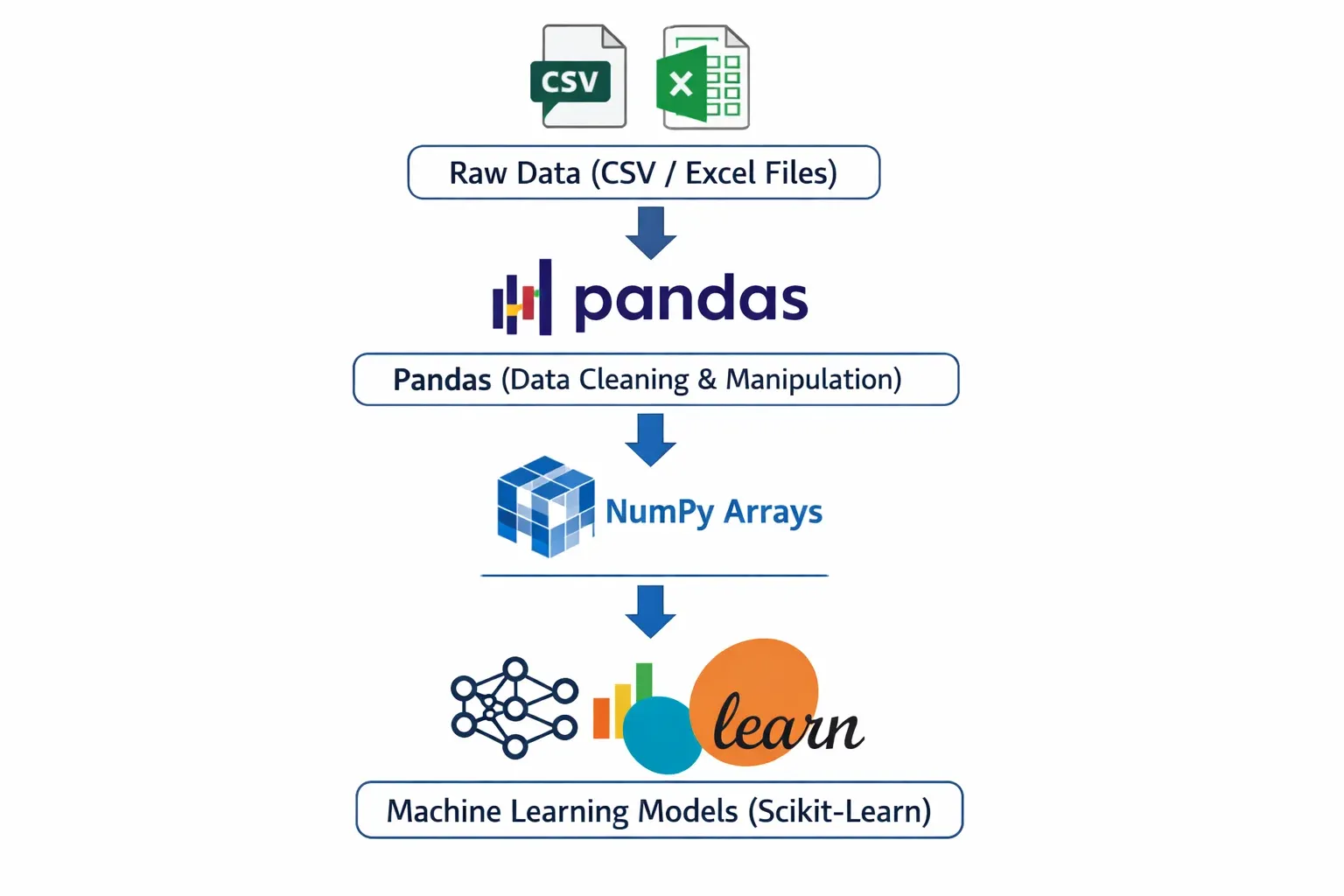
The relationship between NumPy and Pandas is symbiotic. Pandas DataFrames use NumPy arrays as their underlying storage. NumPy's vectorized operations power Pandas computations. And when you need to feed data into a machine learning model (such as those in scikit-learn), you often convert a Pandas DataFrame back into a NumPy array using .values or .to_numpy(). Understanding both libraries is essential for the complete data science workflow.

Practical Code Examples

Example 1: NumPy Arrays for Sales Analysis

Let us start with a practical scenario. Ali runs a small electronics shop in Lahore and wants to analyze his monthly sales data using Python and NumPy.

# Import NumPy with the standard alias 'np'
import numpy as np

# Monthly sales in PKR for 6 months (January to June)
monthly_sales = np.array([125000, 98000, 143000, 167000, 112000, 189000])

# Print the array and its properties
print("Sales Data:", monthly_sales)
print("Data type:", monthly_sales.dtype)
print("Shape:", monthly_sales.shape)
print("Number of elements:", monthly_sales.size)

# Basic statistics — all computed in a single line each
print("\n--- Sales Analysis ---")
print(f"Total Sales (6 months): PKR {monthly_sales.sum():,}")
print(f"Average Monthly Sales: PKR {monthly_sales.mean():,.0f}")
print(f"Best Month Sales: PKR {monthly_sales.max():,}")
print(f"Worst Month Sales: PKR {monthly_sales.min():,}")
print(f"Standard Deviation: PKR {monthly_sales.std():,.0f}")

# Apply a 10% discount using broadcasting — no loop needed!
discounted_sales = monthly_sales * 0.90
print("\nSales after 10% discount:", discounted_sales)

# Find months where sales exceeded PKR 130,000
high_sales_mask = monthly_sales > 130000
print("\nMonths with sales > 130,000 PKR:", monthly_sales[high_sales_mask])

# Calculate cumulative sales month over month
cumulative = np.cumsum(monthly_sales)
print("Cumulative Sales:", cumulative)

# Reshape data into a 2x3 matrix (2 quarters, 3 months each)
quarterly_view = monthly_sales.reshape(2, 3)
print("\nQuarterly View (2 rows = 2 quarters):\n", quarterly_view)
print("Q1 Total: PKR", quarterly_view[0].sum():,)
print("Q2 Total: PKR", quarterly_view[1].sum():,)

Line-by-line explanation:

import numpy as np — Imports the NumPy library. The alias np is a universal convention in the data science community; you will see it in every tutorial, textbook, and Stack Overflow answer.

np.array([...]) — Creates a 1D NumPy array from a Python list. Unlike a Python list, this array is stored as a contiguous block of int64 values in memory.

.dtype, .shape, .size — These are array attributes (not methods — no parentheses needed). They reveal the data type, the dimensions as a tuple, and the total number of elements respectively.

.sum(), .mean(), .max(), .min(), .std() — These are aggregation methods built into NumPy arrays. Each scans the entire array and returns a single result. They are dramatically faster than Python's built-in equivalents on large arrays.

monthly_sales * 0.90 — This is broadcasting in action. NumPy multiplies every single element by 0.90 without any loop. The scalar 0.90 is "broadcast" to match the array's shape.

monthly_sales > 130000 — Creates a boolean mask — an array of True and False values. Passing this mask back into the array (monthly_sales[high_sales_mask]) returns only the elements where the condition is True. This is called boolean indexing.

np.cumsum() — Computes the cumulative sum: each element is the sum of all previous elements plus itself. Useful for running totals.

.reshape(2, 3) — Reorganizes the flat 6-element array into a 2-row, 3-column matrix. The total number of elements must remain the same (2 × 3 = 6). Row index 0 gives the first 3 months (Q1), row index 1 gives the next 3 (Q2).

Example 2: Real-World Application — Student Grade Analysis with Pandas

Now let us tackle a more realistic, multi-column dataset using Pandas. Imagine Fatima is a teaching assistant at a university in Islamabad and has a CSV file of student grades. We will simulate this dataset in code, then perform the kind of analysis she would need to generate a semester report.

import pandas as pd
import numpy as np

# Simulate a student grades dataset
data = {
    'Student_Name': ['Ahmad', 'Fatima', 'Ali', 'Zara', 'Hassan', 
                     'Ayesha', 'Bilal', 'Sara', 'Usman', 'Hira'],
    'City': ['Lahore', 'Karachi', 'Islamabad', 'Lahore', 'Karachi',
             'Islamabad', 'Lahore', 'Karachi', 'Islamabad', 'Lahore'],
    'Maths': [85, 92, 78, 65, 88, 95, 72, 81, 67, 90],
    'Physics': [79, 88, 82, 70, 91, 87, 68, 75, 73, 85],
    'Computer_Science': [95, 98, 90, 80, 85, 99, 88, 92, 76, 97],
    'Attendance': [92, 88, 95, 70, 85, 98, 75, 88, 65, 93]
}

# Create a DataFrame from the dictionary
df = pd.DataFrame(data)

# ---- STEP 1: Basic Exploration ----
print("=== DataFrame Shape ===")
print(f"Rows: {df.shape[0]}, Columns: {df.shape[1]}")

print("\n=== First 5 Rows ===")
print(df.head())

print("\n=== Data Types ===")
print(df.dtypes)

print("\n=== Statistical Summary ===")
print(df.describe())

# ---- STEP 2: Add a calculated column ----
# Calculate each student's average marks across 3 subjects
df['Average_Marks'] = df[['Maths', 'Physics', 'Computer_Science']].mean(axis=1)
df['Average_Marks'] = df['Average_Marks'].round(2)

# Assign grades based on average
def assign_grade(avg):
    if avg >= 90:
        return 'A+'
    elif avg >= 80:
        return 'A'
    elif avg >= 70:
        return 'B'
    elif avg >= 60:
        return 'C'
    else:
        return 'F'

df['Grade'] = df['Average_Marks'].apply(assign_grade)

print("\n=== Student Results ===")
print(df[['Student_Name', 'Average_Marks', 'Grade']].to_string(index=False))

# ---- STEP 3: Filtering ----
# Students who need academic support (average below 75)
at_risk = df[df['Average_Marks'] < 75]
print(f"\n=== Students Needing Support ({len(at_risk)} students) ===")
print(at_risk[['Student_Name', 'City', 'Average_Marks', 'Attendance']])

# ---- STEP 4: GroupBy Analysis ----
city_performance = df.groupby('City')['Average_Marks'].agg(['mean', 'max', 'min', 'count'])
city_performance.columns = ['City_Avg', 'Highest', 'Lowest', 'Students']
city_performance = city_performance.round(2)
print("\n=== Performance by City ===")
print(city_performance)

# ---- STEP 5: Sorting ----
top_students = df.nlargest(3, 'Average_Marks')[['Student_Name', 'City', 'Average_Marks', 'Grade']]
print("\n=== Top 3 Students ===")
print(top_students.to_string(index=False))

# ---- STEP 6: Save results to CSV ----
df.to_csv('student_results.csv', index=False)
print("\n✓ Results saved to 'student_results.csv'")

Detailed explanation:

pd.DataFrame(data) — Creates a DataFrame from a Python dictionary. Dictionary keys become column names; values (lists) become the column data. All lists must be the same length.

df.shape — Returns a tuple (rows, columns). A quick sanity check after loading any dataset.

df.head() — Shows the first 5 rows. Change to df.head(10) for more rows. Equivalent for the end of the dataset: df.tail().

df.dtypes — Shows the data type of each column. object means string data. int64 and float64 are numeric. Knowing this is critical before performing math operations.

df.describe() — A powerful single-line summary: count, mean, standard deviation, min, 25th percentile, median, 75th percentile, and max for every numeric column. Instantly reveals outliers and data quality issues.

df[['Maths', 'Physics', 'Computer_Science']].mean(axis=1) — Selecting multiple columns with double brackets returns a DataFrame. Calling .mean(axis=1) computes the mean across columns (horizontally) for each row. axis=0 would compute the mean down each column (vertically).

df['Average_Marks'].apply(assign_grade) — The .apply() method passes each value in a Series through a function and returns a new Series with the results. It is the Pandas equivalent of Python's map().

df[df['Average_Marks'] < 75] — Boolean indexing in Pandas: the condition inside creates a boolean Series; using it as an index filters to only rows where the condition is True.

df.groupby('City')['Average_Marks'].agg([...]) — Groups the DataFrame by unique values in the City column, then for the Average_Marks column, computes multiple aggregation functions simultaneously. The result is a summary DataFrame indexed by city.

df.nlargest(3, 'Average_Marks') — Efficiently returns the top N rows sorted by a column, without sorting the entire DataFrame. More memory-efficient than df.sort_values().head(n) for large datasets.

df.to_csv('student_results.csv', index=False) — Saves the DataFrame as a CSV file. index=False prevents Pandas from writing the row index numbers as an extra column, which is usually unwanted in output files

Common Mistakes & How to Avoid Them

Mistake 1: Modifying a DataFrame Slice Without Knowing About the SettingWithCopyWarning

This is one of the most confusing errors beginners encounter. When you slice a DataFrame and then try to modify the slice, Pandas may not modify the original DataFrame — and it warns you with a SettingWithCopyWarning.

The wrong way:

import pandas as pd

df = pd.DataFrame({'marks': [55, 72, 88, 45, 91], 'status': ['fail', 'pass', 'pass', 'fail', 'pass']})

# This creates a COPY of the DataFrame, not a view
failing_students = df[df['marks'] < 60]

# Trying to modify the copy — this might not affect the original df
failing_students['status'] = 'needs_support'  # SettingWithCopyWarning!
print(df)  # Original df is likely unchanged!

The correct way — use .copy() or .loc:

# Option 1: Work with an explicit copy when you want a separate object
failing_students = df[df['marks'] < 60].copy()
failing_students['status'] = 'needs_support'  # Safe — modifying the copy
print(failing_students)

# Option 2: Modify the original DataFrame in-place using .loc
df.loc[df['marks'] < 60, 'status'] = 'needs_support'
print(df)  # Original correctly updated

The .loc[row_condition, column_name] accessor is the proper way to filter rows and set column values simultaneously on the original DataFrame. Make this your default approach for conditional assignments.

Mistake 2: Using Python Loops Instead of Vectorized Operations

Coming from a background of regular Python programming, it is tempting to loop through every row of a DataFrame to perform calculations. This works — but it is devastatingly slow on large datasets and completely negates the performance benefits of NumPy and Pandas.

The wrong (slow) way:

import pandas as pd
import time

df = pd.DataFrame({'price_pkr': range(1, 100001), 'quantity': range(1, 100001)})

# Loop-based approach — avoid this!
start = time.time()
revenue = []
for i in range(len(df)):
    revenue.append(df['price_pkr'].iloc[i] * df['quantity'].iloc[i])
df['revenue_loop'] = revenue
print(f"Loop time: {time.time() - start:.3f} seconds")

# Vectorized approach — this is the Pandas way
start = time.time()
df['revenue_vectorized'] = df['price_pkr'] * df['quantity']
print(f"Vectorized time: {time.time() - start:.3f} seconds")

# Results are identical, but the vectorized approach is 50-200x faster

On 100,000 rows, the loop typically takes 1–3 seconds while the vectorized operation takes milliseconds. On a real-world dataset with millions of rows (think Karachi port shipping records or telecom subscriber data), this difference becomes the distinction between an analysis that finishes in seconds versus one that takes hours.

The rule: if you find yourself writing for i in range(len(df)):, stop and think whether there is a vectorized alternative using column arithmetic, .apply(), or a NumPy ufunc. There almost always is.

Practice Exercises

Exercise 1: NumPy Array Operations on Cricket Statistics

Problem: Pakistan's cricket team played 8 ODI matches this year. Their scores were: 312, 267, 298, 341, 185, 278, 320, 255. Using NumPy, write a script that:

1. Creates a NumPy array of these scores
2. Calculates total runs, average score, and standard deviation
3. Finds how many matches they scored above the average
4. Normalizes the scores to a 0–1 scale (hint: (x - min) / (max - min))
5. Determines the percentage difference of each match from the overall average

Solution:

import numpy as np

# Step 1: Create array
scores = np.array([312, 267, 298, 341, 185, 278, 320, 255])

# Step 2: Basic statistics
total = scores.sum()
average = scores.mean()
std_dev = scores.std()
print(f"Total Runs: {total}")
print(f"Average Score: {average:.2f}")
print(f"Standard Deviation: {std_dev:.2f}")

# Step 3: Matches above average
above_avg = scores[scores > average]
print(f"\nMatches above average ({average:.0f}): {len(above_avg)}")
print(f"Scores above average: {above_avg}")

# Step 4: Normalize scores to 0-1 range
normalized = (scores - scores.min()) / (scores.max() - scores.min())
print(f"\nNormalized scores: {normalized.round(3)}")

# Step 5: Percentage difference from average
pct_diff = ((scores - average) / average) * 100
labels = ['Match ' + str(i+1) for i in range(len(scores))]
for label, score, pct in zip(labels, scores, pct_diff):
    direction = "above" if pct > 0 else "below"
    print(f"{label}: {score} runs ({abs(pct):.1f}% {direction} average)")

Expected Output Highlights: Total runs around 2,456. Average around 307. Five matches above average (scores of 312, 341, 320, 298, and 278 if average ~307). The lowest normalized score corresponds to the 185-run match (0.0), and the highest to 341 (1.0).

Exercise 2: Pandas Data Cleaning and Analysis — Karachi Market Prices

Problem: You have received a messy dataset of fruit prices from different markets in Karachi. The data has missing values, inconsistent capitalization, and duplicate entries. Clean it and perform a market analysis.

import pandas as pd
import numpy as np

# Messy raw data (simulating real-world data quality issues)
raw_data = {
    'Fruit': ['Apple', 'apple', 'Mango', 'Banana', 'MANGO', 'Orange', 
              'Banana', 'Apple', 'Grape', 'Orange'],
    'Market': ['Empress Market', 'Sunday Bazaar', 'Empress Market', 'Sunday Bazaar',
               'Sunday Bazaar', 'Empress Market', 'Empress Market', 'Sunday Bazaar',
               'Empress Market', 'Sunday Bazaar'],
    'Price_PKR_per_kg': [250, 230, 180, 60, None, 120, 55, 245, 350, 115],
    'Stock_kg': [50, 30, 100, 200, 80, 75, None, 45, 20, 90]
}

df = pd.DataFrame(raw_data)
print("=== Raw Data ===")
print(df)
print(f"\nMissing values:\n{df.isnull().sum()}")

# ---- CLEANING STEPS ----

# Step 1: Standardize fruit names to title case
df['Fruit'] = df['Fruit'].str.title()
print("\nAfter title-casing fruit names:")
print(df['Fruit'].unique())

# Step 2: Fill missing Price with median price for that fruit
df['Price_PKR_per_kg'] = df.groupby('Fruit')['Price_PKR_per_kg'].transform(
    lambda x: x.fillna(x.median())
)

# Step 3: Fill missing Stock with overall median
df['Stock_kg'] = df['Stock_kg'].fillna(df['Stock_kg'].median())

# Step 4: Remove duplicate fruit-market combinations, keep lowest price
df = df.sort_values('Price_PKR_per_kg').drop_duplicates(
    subset=['Fruit', 'Market'], keep='first'
).reset_index(drop=True)

print("\n=== Cleaned Data ===")
print(df)

# ---- ANALYSIS ----

# Calculate inventory value
df['Inventory_Value_PKR'] = df['Price_PKR_per_kg'] * df['Stock_kg']

# Market comparison
market_summary = df.groupby('Market').agg(
    Total_Inventory_Value=('Inventory_Value_PKR', 'sum'),
    Avg_Price=('Price_PKR_per_kg', 'mean'),
    Unique_Fruits=('Fruit', 'count')
).round(2)

print("\n=== Market Summary ===")
print(market_summary)

# Most affordable fruit overall
cheapest = df.loc[df['Price_PKR_per_kg'].idxmin()]
print(f"\nMost Affordable: {cheapest['Fruit']} at PKR {cheapest['Price_PKR_per_kg']}/kg from {cheapest['Market']}")

What this exercise teaches: Real-world datasets are never clean. This example covers str.title() for text normalization, groupby().transform() for group-aware missing value imputation (filling missing prices with the median for that specific fruit), drop_duplicates() for deduplication, and chained aggregations for business insights.

Frequently Asked Questions

What is the difference between NumPy and Pandas in Python machine learning?

NumPy provides the low-level numerical computing infrastructure — primarily the ndarray for storing and operating on homogeneous numerical data at high speed. Pandas builds on NumPy to provide higher-level, user-friendly tools for working with heterogeneous, labeled, tabular data that resembles spreadsheets. In a typical machine learning workflow, you use Pandas to load, clean, and explore data, then convert to NumPy arrays to feed into model training functions from libraries like scikit-learn.

How do I install NumPy and Pandas in Pakistan without a VPN?

Both libraries are available through PyPI (Python Package Index) and are accessible without any VPN from any Pakistani internet connection. Simply open your terminal or command prompt and run pip install numpy pandas. If you are using Anaconda (recommended), these libraries come pre-installed. You can also use Google Colab — a free, browser-based Jupyter Notebook environment that has NumPy and Pandas pre-installed and requires no local setup at all.

How long does it take to learn NumPy and Pandas for machine learning?

With consistent daily practice of 1–2 hours, most intermediate Python learners become productive with NumPy and Pandas within 3–6 weeks. The core 20% of features (array creation, indexing, filtering, groupby, merge, handling missing data) covers 80% of real-world data science tasks. Building projects with real Pakistani datasets — such as PSX stock data, HEC enrollment statistics, or NEPRA electricity consumption data — accelerates learning significantly faster than working through abstract exercises alone.

What is the best free resource to practice Pandas in Pakistan?

Google Colab is unquestionably the most accessible tool: it is free, runs in any browser, requires no installation, and provides free GPU access for machine learning. For datasets, Kaggle offers thousands of free public datasets, and Pakistani government portals like data.gov.pk provide local datasets. For structured learning, theiqra.edu.pk's Pandas Complete Course offers step-by-step tutorials specifically designed for Pakistani learners.

Is Python machine learning a good career choice in Pakistan?

The demand for Python machine learning skills in Pakistan is growing significantly. Companies in fintech (JazzCash, Easypaisa), e-commerce (Daraz), telecommunications (Jazz, Telenor Pakistan), and outsourced software development actively seek data scientists and ML engineers. Freelancing platforms like Upwork and Fiverr show consistent demand for Pakistani Python data scientists on international projects. Starting salaries for junior data science roles in Pakistan range from PKR 80,000 to PKR 150,000/month, with senior practitioners earning considerably more or scaling via international freelancing rates.

Summary & Key Takeaways

Here is a concise recap of everything covered in this tutorial:

• NumPy's ndarray is the cornerstone of numerical computing in Python — it provides vectorized operations that are 50–200x faster than Python loops, making it essential for any machine learning project that works with large numerical datasets.
• Pandas DataFrame and Series provide a labeled, tabular data structure that makes loading, cleaning, filtering, grouping, and summarizing real-world datasets intuitive and expressive — bridging the gap between raw data files and machine learning-ready arrays.
• Always prefer vectorized operations over explicit Python loops when working with NumPy arrays or Pandas columns. Column arithmetic, boolean indexing, .apply(), and .groupby() aggregations are your tools of choice.
• Data cleaning is 70–80% of real-world data science work. Pandas provides the tools for it: str.title() for text standardization, .fillna() for missing values, .drop_duplicates() for deduplication, and .loc for safe conditional assignments.
• The SettingWithCopyWarning exists for a reason — always use .loc[condition, column] for in-place DataFrame modifications and .copy() when you intentionally want a separate object, to avoid subtle bugs in your data pipelines.
• NumPy and Pandas work together seamlessly. Pandas DataFrames are backed by NumPy arrays. Converting with .to_numpy() is frictionless, making it easy to move data from Pandas exploration into scikit-learn model training.

Next Steps & Related Tutorials

Now that you have a solid foundation in NumPy and Pandas, here is how to continue your Python machine learning journey on theiqra.edu.pk:

Matplotlib and Seaborn Data Visualization Tutorial — Once your data is clean and analyzed, the next step is visualizing it. This tutorial teaches you to create bar charts, scatter plots, heatmaps, and distribution plots that bring your Pandas DataFrames to life — an essential skill for communicating findings to non-technical stakeholders.

Scikit-Learn Machine Learning for Beginners — Now that you know how to prepare data with NumPy and Pandas, this tutorial shows you how to build your first classification and regression models using scikit-learn — Pakistan's most in-demand ML skill in the job market right now.

Python Data Cleaning: Handling Missing Values and Outliers — Go deeper into real-world data preparation challenges. This intermediate tutorial covers advanced imputation strategies, outlier detection using the IQR method, and building reusable data cleaning pipelines — the kind of work that takes up the majority of a professional data scientist's time.

Time Series Analysis with Pandas — Pakistani datasets ranging from PSX stock prices to electricity load data from NEPRA are time series in nature. This tutorial explores Pandas' powerful DatetimeIndex, resampling, rolling windows, and seasonal decomposition to extract meaningful trends from temporal data.

Happy coding! If you found this tutorial helpful, share it with your study group or classmates at university. The more of us who build these skills together, the stronger Pakistan's tech ecosystem becomes. 🇵🇰

Written for theiqra.edu.pk — Pakistan's Programming Learning Community