Reinforcement Learning Q Learning & OpenAI Gym Guide
Introduction
Imagine you are teaching a robot to play a video game — not by programming every move manually, but by letting it learn from experience, just like a child learns to walk by trial and error. That is the core idea behind Reinforcement Learning (RL), one of the most powerful and exciting branches of machine learning today.
In this reinforcement learning tutorial, you will master Q-Learning — a foundational RL algorithm — and learn to use OpenAI Gym, the most popular Python toolkit for building and testing RL environments. By the end, you will have trained an AI agent to balance a pole in the classic CartPole simulation, a satisfying and career-building achievement.
For Pakistani students studying machine learning in Lahore, Karachi, or Islamabad, this is the gateway to some of the most in-demand skills in the tech industry. Companies building autonomous systems, game AIs, trading bots, and robotics all rely on reinforcement learning. The global AI market is growing rapidly, and engineers who understand RL are exceptionally well-positioned — whether working at a local startup or a multinational firm.
By the end of this guide you will be able to:
- Explain the core components of a reinforcement learning system
- Build and run OpenAI Gym environments in Python
- Implement a Q-Learning algorithm from scratch
- Train an agent to solve the CartPole-v1 environment
- Avoid the most common pitfalls that trip up beginners
Prerequisites
Before diving into this q learning python tutorial, make sure you are comfortable with the following:
- Python 3.8+ — variables, loops, functions, and classes
- NumPy — array creation and manipulation (we use it heavily for the Q-table)
- Basic Machine Learning concepts — you should understand what a model, training, and loss mean at a high level. If not, start with our Machine Learning Basics tutorial on theiqra.edu.pk
- Basic Probability — understanding of probability distributions and random choices
- pip / virtual environments — you need to install packages
You do not need prior deep learning experience. Q-Learning is mathematically accessible and a great standalone entry point into RL.
Installation: Run the following in your terminal before proceeding:
pip install gymnasium numpy matplotlib
Note: As of 2023, OpenAI Gym has been superseded by Gymnasium (maintained by the Farama Foundation), which is the package we use throughout this tutorial. The API is almost identical to OpenAI Gym.
Core Concepts & Explanation
The Agent-Environment Loop
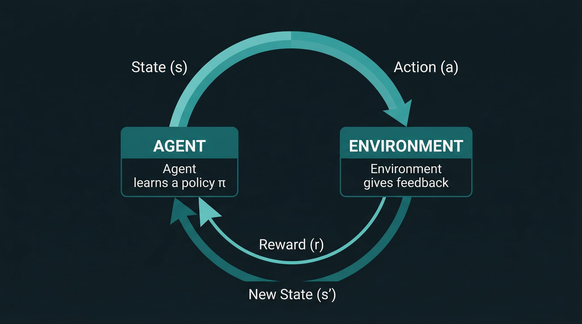
Every reinforcement learning problem is built around one central idea: an agent interacts with an environment over time, trying to maximize cumulative reward.
Think of it this way: Fatima is playing a mobile game. She (the agent) looks at the game screen (the state), decides to swipe left (the action), and the game either gives her points or takes them away (the reward), then shows a new screen (the next state). Her goal is to earn as many points as possible over the entire game session (maximize return).
In formal terms, RL involves these five components:
| Component | Symbol | Description |
|---|---|---|
| State | s | A description of the environment at a given moment |
| Action | a | A choice the agent makes in response to a state |
| Reward | r | A scalar feedback signal from the environment |
| Policy | π | The strategy the agent uses to pick actions |
| Value | V(s) or Q(s,a) | Expected future reward from a state or state-action pair |
The agent follows a cycle: observe state → pick action → receive reward → observe new state → repeat. The goal is to learn a policy — a mapping from states to actions — that maximises the total reward over time.
Pakistani analogy: Think of Ahmad running a small e-commerce shop on Daraz.pk. Each day he decides how much inventory to order (action), based on current stock levels and demand (state). If he orders too little, he loses sales (negative reward); if too much, he loses money on storage (negative reward). Over months, Ahmad learns the optimal ordering policy — that is reinforcement learning in a real business context.
Q-Learning: Teaching an Agent with a Table
Q-Learning is a model-free, off-policy RL algorithm. "Model-free" means the agent does not build an internal map of the environment — it simply learns from raw experience. "Off-policy" means it can learn from actions it did not actually take, which makes it very data-efficient.
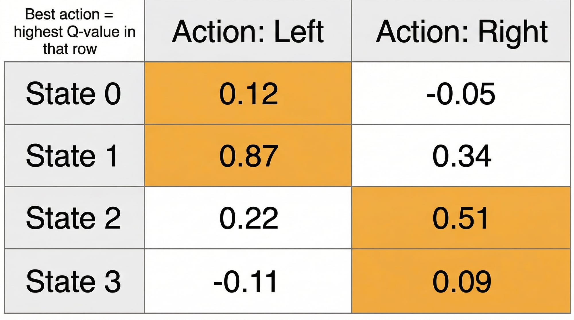
The heart of Q-Learning is the Q-table: a lookup table where rows are states, columns are actions, and each cell holds a Q-value — the expected total reward for taking that action in that state and then following the optimal policy afterward.
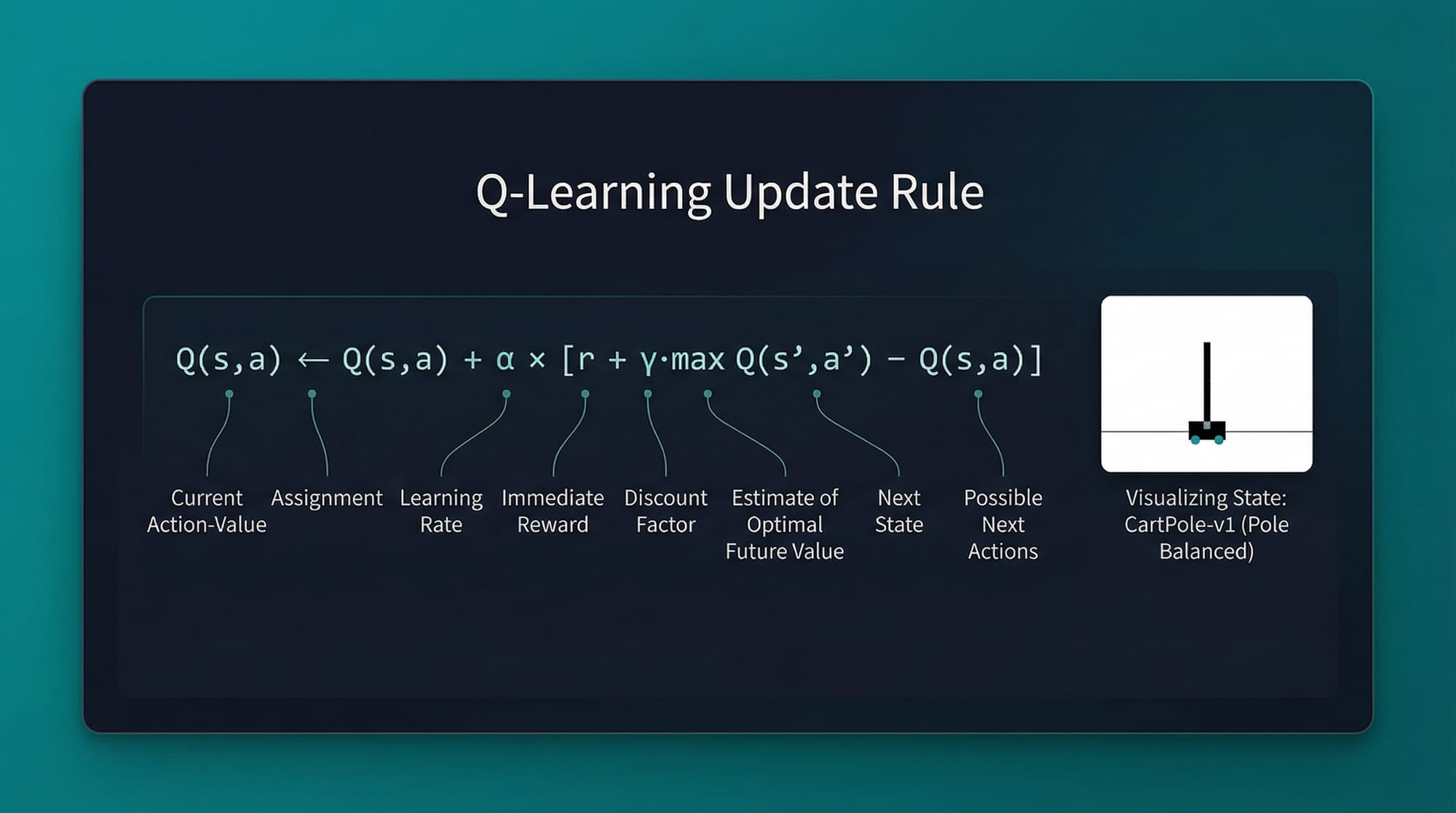
The Q-Learning Update Rule is the single formula you must understand:
Q(s, a) ← Q(s, a) + α × [r + γ × max(Q(s', a')) − Q(s, a)]
Let us break this down piece by piece:
- Q(s, a) — the current estimate of value for taking action
ain states - α (alpha) — the learning rate (typically 0.1–0.5). How fast the agent updates its beliefs
- r — the immediate reward received after taking action
a - γ (gamma) — the discount factor (0 to 1). How much the agent values future rewards vs. immediate ones. A value of 0.99 means the agent cares a lot about the future.
- max(Q(s', a')) — the best possible Q-value in the next state
s'. This is the "bootstrapped" estimate of future value. - The term in brackets
[r + γ × max(...) − Q(s, a)]is called the TD error (Temporal Difference error) — how wrong our current estimate was.
Intuition: If the agent took an action and got a better-than-expected reward, increase the Q-value for that (state, action) pair. If the reward was worse than expected, decrease it. Over thousands of episodes, the Q-values converge to the optimal ones.
Exploration vs. Exploitation
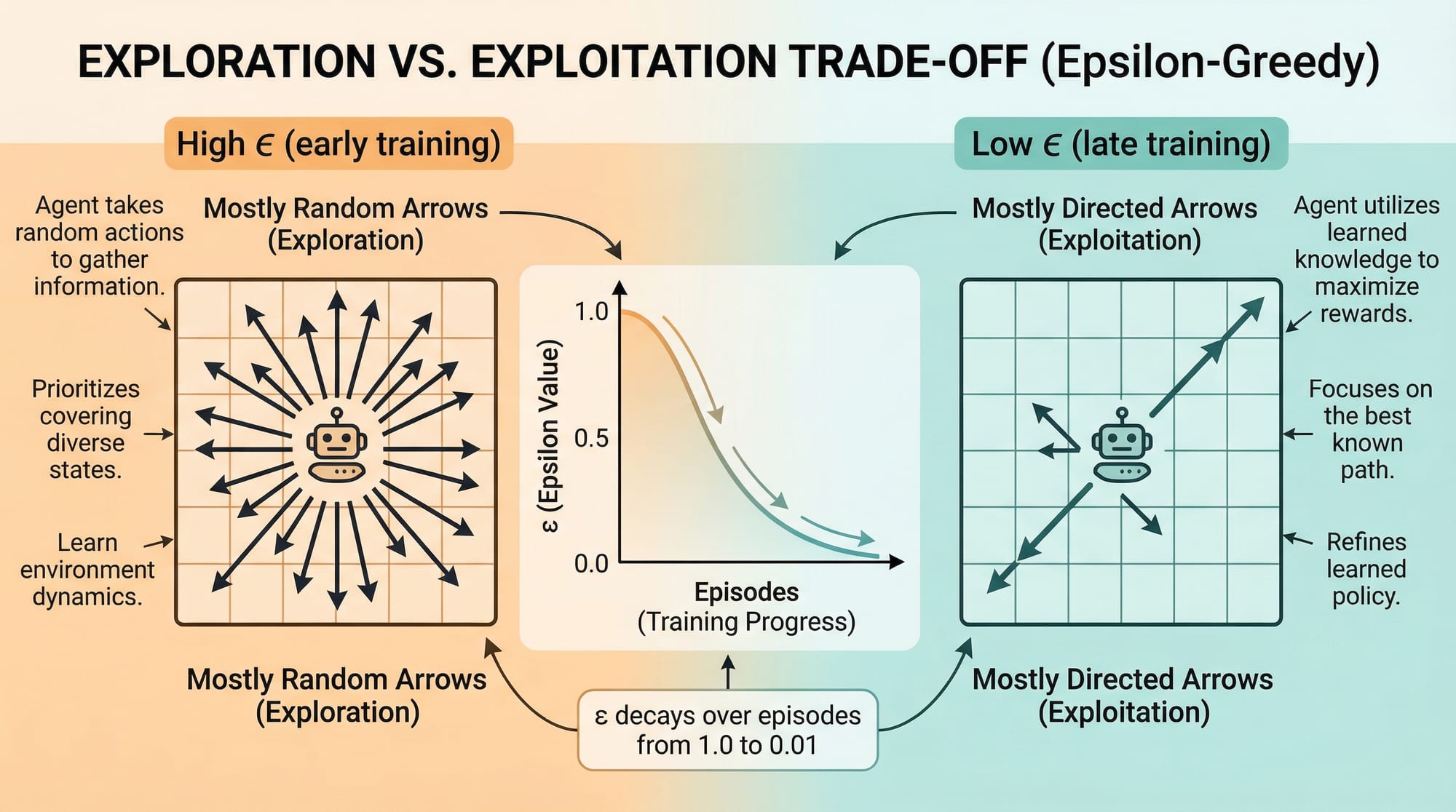
One of the most important challenges in RL is the exploration-exploitation trade-off:
- Exploitation: Use what you already know — always pick the action with the highest current Q-value
- Exploration: Try random actions to discover potentially better strategies
If Ali (our agent) only exploits, he might get stuck in a suboptimal strategy forever. If he only explores, he never actually uses what he has learned.
The most common solution is the epsilon-greedy policy:
if random.uniform(0, 1) < epsilon:
    action = env.action_space.sample()   # Explore: pick random action
else:
    action = np.argmax(Q[state])          # Exploit: pick best known action
We typically start with a high epsilon (e.g., 1.0 = 100% random) and decay it over time as the agent learns more, gradually shifting from exploration to exploitation.
Practical Code Examples
Example 1: Setting Up OpenAI Gym and Exploring an Environment
Before training any agent, you need to understand the environment you are working with. Let us explore the CartPole-v1 environment — a classic RL benchmark where the goal is to balance a pole on a moving cart.
import gymnasium as gym   # Line 1: Import Gymnasium (the modern OpenAI Gym)
import numpy as np        # Line 2: Import NumPy for numerical operations

# Line 4: Create the CartPole environment
# render_mode="human" opens a visual window (use "rgb_array" for headless servers)
env = gym.make("CartPole-v1", render_mode="human")

# Line 8: Reset the environment to get the initial state
# seed=42 ensures reproducibility (Ahmad and Fatima get the same starting state)
state, info = env.reset(seed=42)

print(f"Observation space: {env.observation_space}")
# Output: Box([-4.8, -inf, -0.42, -inf], [4.8, inf, 0.42, inf], (4,), float32)
# This means the state is a 4-element array: [cart_pos, cart_vel, pole_angle, pole_vel]

print(f"Action space: {env.action_space}")
# Output: Discrete(2)
# This means there are only 2 actions: 0 (push left) or 1 (push right)

print(f"Initial state: {state}")
# Example output: [ 0.0273  -0.0435  0.0477  -0.0619]

# Line 20: Run one episode with RANDOM actions to see how the environment works
total_reward = 0

for step in range(200):                         # Line 23: Run up to 200 steps
    action = env.action_space.sample()          # Line 24: Pick a completely random action

    # Line 26: Take the action. Returns:
    # - next_state: new observation after the action
    # - reward: +1.0 for every step the pole stays up
    # - terminated: True if pole fell or cart went off screen
    # - truncated: True if episode hit the 500-step limit
    # - info: extra diagnostic information (usually empty here)
    next_state, reward, terminated, truncated, info = env.step(action)

    total_reward += reward                      # Line 33: Accumulate reward

    if terminated or truncated:                 # Line 35: End episode if done
        print(f"Episode ended at step {step + 1}, Total reward: {total_reward}")
        break

env.close()    # Line 39: Always close the environment when done
Key insight: With random actions, the pole typically falls within 10–20 steps, earning a reward of 10–20. A trained Q-Learning agent should consistently achieve 200+ steps (the maximum).
Example 2: Real-World Application — Training a Q-Learning Agent on CartPole
Now we build the full Q-Learning training loop. Because CartPole has a continuous observation space (infinite possible states), we first need to discretize it into a finite number of bins so we can build a Q-table.
import gymnasium as gym
import numpy as np
import matplotlib.pyplot as plt

# ─── HYPERPARAMETERS ──────────────────────────────────────────────────────────
EPISODES        = 5000      # Total training episodes (like 5000 practice games)
LEARNING_RATE   = 0.1       # Alpha: how fast we update Q-values (0.1 is conservative)
DISCOUNT_FACTOR = 0.99      # Gamma: we care a lot about future rewards
EPSILON_START   = 1.0       # Start fully exploring (100% random actions)
EPSILON_END     = 0.01      # Minimum exploration rate (always keep 1% randomness)
EPSILON_DECAY   = 0.995     # Multiply epsilon by this each episode (slow decay)
N_BINS          = 20        # Number of discrete bins per continuous dimension

# ─── ENVIRONMENT SETUP ────────────────────────────────────────────────────────
env = gym.make("CartPole-v1")   # No render during training for speed

# ─── DISCRETIZATION SETUP ─────────────────────────────────────────────────────
# CartPole state: [cart_position, cart_velocity, pole_angle, pole_angular_velocity]
# We clip velocities because they are theoretically infinite; in practice they stay small
bins = [
    np.linspace(-4.8,  4.8,   N_BINS),   # Cart position: -4.8m to +4.8m
    np.linspace(-4.0,  4.0,   N_BINS),   # Cart velocity (clipped): -4 to +4
    np.linspace(-0.42, 0.42,  N_BINS),   # Pole angle: -0.42 to +0.42 radians
    np.linspace(-4.0,  4.0,   N_BINS),   # Pole angular velocity (clipped): -4 to +4
]

def discretize(state):
    """Convert a continuous state into a discrete tuple index for the Q-table."""
    state_idx = []
    for i, val in enumerate(state):
        # np.digitize returns which bin the value falls into
        idx = np.digitize(val, bins[i]) - 1          # -1 to make 0-indexed
        idx = np.clip(idx, 0, N_BINS - 1)            # Ensure index stays in range
        state_idx.append(idx)
    return tuple(state_idx)    # Return as a tuple so it can index the Q-table

# ─── Q-TABLE INITIALIZATION ───────────────────────────────────────────────────
# Shape: (N_BINS, N_BINS, N_BINS, N_BINS, 2)
# One dimension per state feature, last dimension for 2 possible actions
q_table = np.zeros([N_BINS] * 4 + [env.action_space.n])
# Starting all Q-values at 0 means the agent initially has no preference

# ─── TRAINING LOOP ────────────────────────────────────────────────────────────
epsilon        = EPSILON_START
rewards_log    = []    # Track rewards per episode for plotting

for episode in range(EPISODES):
    state_cont, _ = env.reset()          # Get continuous state
    state         = discretize(state_cont)  # Convert to discrete index
    total_reward  = 0
    done          = False

    while not done:
        # ── EPSILON-GREEDY ACTION SELECTION ──
        if np.random.uniform(0, 1) < epsilon:
            action = env.action_space.sample()    # EXPLORE: random action
        else:
            action = np.argmax(q_table[state])    # EXPLOIT: best known action

        # ── TAKE ACTION, OBSERVE OUTCOME ──
        next_state_cont, reward, terminated, truncated, _ = env.step(action)
        next_state = discretize(next_state_cont)
        done       = terminated or truncated

        # ── Q-LEARNING UPDATE RULE ──
        current_q   = q_table[state][action]
        best_next_q = np.max(q_table[next_state])    # max Q-value in next state

        # The Bellman equation: blend current estimate with new TD target
        td_target   = reward + DISCOUNT_FACTOR * best_next_q * (not done)
        td_error    = td_target - current_q
        q_table[state][action] += LEARNING_RATE * td_error

        state        = next_state     # Move to next state
        total_reward += reward

    # ── DECAY EPSILON AFTER EACH EPISODE ──
    epsilon = max(EPSILON_END, epsilon * EPSILON_DECAY)
    rewards_log.append(total_reward)

    # ── PROGRESS REPORTING ──
    if (episode + 1) % 500 == 0:
        avg_reward = np.mean(rewards_log[-500:])
        print(f"Episode {episode + 1:5d} | Avg Reward (last 500): {avg_reward:.1f} | ε: {epsilon:.4f}")

env.close()

# ─── PLOT TRAINING PROGRESS ───────────────────────────────────────────────────
plt.figure(figsize=(10, 5))
plt.plot(rewards_log, alpha=0.3, color="steelblue", label="Episode reward")
# Smooth with rolling average to see the trend
rolling_avg = np.convolve(rewards_log, np.ones(100)/100, mode="valid")
plt.plot(rolling_avg, color="crimson", linewidth=2, label="100-ep rolling avg")
plt.axhline(y=195, color="green", linestyle="--", label="Solved threshold (195)")
plt.xlabel("Episode")
plt.ylabel("Total Reward")
plt.title("Q-Learning Training on CartPole-v1 | theiqra.edu.pk")
plt.legend()
plt.tight_layout()
plt.savefig("cartpole_training.png", dpi=150)
plt.show()
print("Training complete! Model saved to cartpole_training.png")
Expected output after 5000 episodes:
Episode   500 | Avg Reward (last 500):  42.3 | ε: 0.0821
Episode  1000 | Avg Reward (last 500):  89.7 | ε: 0.0067
Episode  1500 | Avg Reward (last 500): 154.2 | ε: 0.0100
Episode  2000 | Avg Reward (last 500): 187.6 | ε: 0.0100
Episode  5000 | Avg Reward (last 500): 198.4 | ε: 0.0100
The agent goes from ~10 (random) to ~198 (near-perfect). CartPole is considered "solved" when the average reward over 100 consecutive episodes exceeds 195.
Common Mistakes & How to Avoid Them
Mistake 1: Not Decaying Epsilon (Staying in Exploration Mode Forever)
A very common mistake is setting a fixed, high epsilon (like 0.5) throughout training. If the agent keeps exploring randomly even after it has learned something, it never converges to a good policy.
Wrong approach:
EPSILON = 0.5 # Fixed — agent is always 50% random, even after 5000 episodes
Correct approach:
epsilon = 1.0          # Start fully exploratory
EPSILON_DECAY = 0.995  # Multiply each episode
EPSILON_MIN   = 0.01   # Never go below 1% random

# After each episode:
epsilon = max(EPSILON_MIN, epsilon * EPSILON_DECAY)
Why it matters: After ~1000 episodes, a well-trained agent should exploit its knowledge ~99% of the time. Keeping epsilon high wastes episodes on random behavior and makes training curves noisy and flat.
Mistake 2: Using Too Few or Too Many Discretization Bins
When discretizing a continuous state space, the number of bins is a critical hyperparameter.
Too few bins (e.g., N_BINS = 5):
# Problem: Many distinct physical states map to the same Q-table entry.
# The agent cannot distinguish between a pole at 5° and 20° — both are "bin 3".
# Result: The agent learns a coarse, inaccurate policy.
bins = [np.linspace(-4.8, 4.8, 5), ...]  # Too coarse
Too many bins (e.g., N_BINS = 100):
# Problem: The Q-table has 100^4 × 2 = 200,000,000 entries.
# Most entries are never visited during training — the table stays mostly zeros.
# Result: Extremely slow learning, massive memory usage.
bins = [np.linspace(-4.8, 4.8, 100), ...]  # Memory: ~1.5 GB
Sweet spot for CartPole:
N_BINS = 20 # Q-table has 20^4 × 2 = 320,000 entries — fast and accurate
Rule of thumb: Start with 10–30 bins. Monitor the training curve. If the agent plateaus early, try more bins. If training is slow, try fewer.
Practice Exercises
Exercise 1: Evaluate Your Trained Agent
Problem: After training, you need to measure how well the agent actually performs. Write a function evaluate_agent(q_table, env, n_episodes=100) that runs the trained agent (with epsilon=0, i.e., pure exploitation) for n_episodes episodes and prints the mean and standard deviation of the total reward.
Solution:
def evaluate_agent(q_table, env, n_episodes=100):
    """Evaluate a trained Q-Learning agent with no exploration."""
    rewards = []

    for ep in range(n_episodes):
        state_cont, _ = env.reset()
        state = discretize(state_cont)   # Use the discretize function from above
        total_reward = 0
        done = False

        while not done:
            action = np.argmax(q_table[state])   # Pure exploitation: no randomness
            next_state_cont, reward, terminated, truncated, _ = env.step(action)
            state = discretize(next_state_cont)
            total_reward += reward
            done = terminated or truncated

        rewards.append(total_reward)

    mean_r = np.mean(rewards)
    std_r  = np.std(rewards)
    print(f"Evaluation over {n_episodes} episodes:")
    print(f"  Mean Reward: {mean_r:.2f}")
    print(f"  Std Deviation: {std_r:.2f}")
    print(f"  Solved: {'Yes ✅' if mean_r >= 195 else 'Not yet ❌'}")
    return mean_r, std_r

# Usage (after training):
eval_env = gym.make("CartPole-v1")
evaluate_agent(q_table, eval_env, n_episodes=100)
eval_env.close()
Exercise 2: Try a Different Gym Environment — MountainCar-v0
Problem: Apply the same Q-Learning code to a new environment: MountainCar-v0. In this environment, a car must drive up a mountain by building momentum. The state is [position, velocity] (2D instead of 4D), and the action space has 3 choices: push left (0), do nothing (1), push right (2). Adapt the discretization code and Q-table shape for this new environment. Use N_BINS=40 for better resolution.
Solution skeleton:
import gymnasium as gym
import numpy as np

env  = gym.make("MountainCar-v0")

N_BINS = 40

# MountainCar state bounds are well-defined; no clipping needed
bins = [
    np.linspace(-1.2,   0.6,  N_BINS),   # Position: -1.2 to 0.6
    np.linspace(-0.07,  0.07, N_BINS),   # Velocity: -0.07 to 0.07
]

def discretize_mc(state):
    """Discretize MountainCar's 2D continuous state."""
    return tuple(
        np.clip(np.digitize(state[i], bins[i]) - 1, 0, N_BINS - 1)
        for i in range(2)
    )

# Q-table shape: (40, 40, 3) — 40×40 states, 3 possible actions
q_table_mc = np.zeros([N_BINS, N_BINS, env.action_space.n])

# Tip: MountainCar is harder than CartPole. Use a higher discount (0.99)
# and more episodes (10,000+). The reward is -1 per step until the car reaches
# the goal (position >= 0.5), so the agent must learn to build momentum first.

print("Q-table shape:", q_table_mc.shape)    # (40, 40, 3)
print("Now apply the same training loop from Example 2 — good luck! 🎯")

env.close()
Frequently Asked Questions
What is the difference between Q-Learning and Deep Q-Learning (DQN)?
Q-Learning uses a lookup table (Q-table) to store values for every (state, action) pair. This works well for small, discrete environments but becomes impossible when the state space is very large or continuous. Deep Q-Learning (DQN), popularized by DeepMind, replaces the Q-table with a neural network that can approximate Q-values for any state. This allows RL to scale to complex tasks like playing Atari games directly from pixel inputs. Our Deep Learning tutorial on theiqra.edu.pk covers the neural network fundamentals you need before tackling DQN.
How do I choose the right learning rate and discount factor?
The learning rate (α) controls how aggressively the agent updates its beliefs. Values between 0.05 and 0.3 work well for most tabular problems. Too high (e.g., 0.9) causes instability; too low (e.g., 0.001) makes learning very slow. The discount factor (γ) controls the agent's time horizon. Use 0.99 for tasks where future rewards matter a lot (like CartPole, where surviving longer is always better). Use lower values like 0.9 for tasks with very long episodes where distant rewards are hard to credit. Start with α=0.1 and γ=0.99 and adjust based on your training curve.
Why does my CartPole agent learn well but then forget?
This phenomenon is called catastrophic forgetting or policy instability, and it is common in tabular Q-Learning with discretization. When the Q-table updates for one state accidentally override useful values for nearby states (due to overlapping bins), performance can drop. Solutions include: reducing the learning rate, using a finer bin grid, switching to a neural network (DQN) which generalises better across states, or using experience replay to stabilise training.
Is OpenAI Gym still being maintained in 2024?
The original OpenAI Gym repository is no longer actively maintained by OpenAI. The community forked it as Gymnasium (by the Farama Foundation), which is the current standard used in research and education. The API is nearly identical — just change import gym to import gymnasium as gym and update env.step() to handle the 5-value return tuple (obs, reward, terminated, truncated, info) instead of the old 4-value tuple. All code in this tutorial uses Gymnasium.
What real-world applications use Q-Learning and RL in Pakistan's tech industry?
Q-Learning and its deep variants power many real-world products. In Pakistan's growing tech sector, RL is being explored for: algorithmic trading on the Pakistan Stock Exchange (PSX) — agents that learn buy/sell policies to maximise PKR returns; logistics optimisation for companies like Airlift-style platforms — routing agents that minimise delivery time; game AI development at local studios; telecom network optimisation — agents that adjust bandwidth allocation dynamically; and smart energy management in industrial settings. As AI adoption accelerates across Karachi, Lahore, and Islamabad, RL skills will become increasingly valuable for Pakistani engineers.
Summary & Key Takeaways
- Reinforcement Learning is a paradigm where an agent learns by interacting with an environment, receiving rewards for good actions and penalties for bad ones — no labelled dataset required.
- Q-Learning stores the expected future reward for each (state, action) pair in a Q-table and updates it using the Bellman equation:
Q(s,a) ← Q(s,a) + α[r + γ·maxQ(s',a') − Q(s,a)]. - Gymnasium (the modern OpenAI Gym) provides a standardised Python interface for dozens of RL environments, from simple CartPole to complex robotics simulations.
- The epsilon-greedy strategy balances exploration (trying new things) and exploitation (using what you know), with epsilon decaying over time as the agent becomes more confident.
- Discretization is essential when applying tabular Q-Learning to continuous state spaces — the number of bins is a critical hyperparameter that trades off accuracy against memory and speed.
- Q-Learning is the foundation for more advanced algorithms like DQN, A3C, PPO, and SAC, which power modern AI applications in gaming, robotics, and finance.
Next Steps & Related Tutorials
You have taken a major step into one of the most exciting areas of AI. Here is where to go next on theiqra.edu.pk:
- Deep Learning Fundamentals — Learn neural networks from scratch. This is the prerequisite for Deep Q-Networks (DQN), which can solve far more complex problems than tabular Q-Learning.
- Machine Learning Basics with Scikit-Learn — If some concepts in this tutorial felt unfamiliar, reinforce your foundations with supervised and unsupervised learning before returning to RL.
- NumPy for Data Science — A deeper dive into NumPy arrays, broadcasting, and vectorised operations. Since the Q-table is a NumPy array, mastering NumPy will help you write faster, cleaner RL code.
- Python OOP and Class Design — As your RL projects grow, you will want to encapsulate your agent, environment, and training loop into clean Python classes. This tutorial teaches you exactly that.
Written for theiqra.edu.pk — Pakistan's community for aspiring programmers. Happy coding! 🚀
Test Your Python Knowledge!
Finished reading? Take a quick quiz to see how much you've learned from this tutorial.